Let’s start at the beginning. Or, close to it.
Here at the start, we’re going to describe the process at a high level and establish some terms. We’ll then go a little bit deeper and put some additional detail on those terms.
We have two computers, Computer A and Computer B. An application on Computer A needs to send some data to the IP address 10.200.200.20.
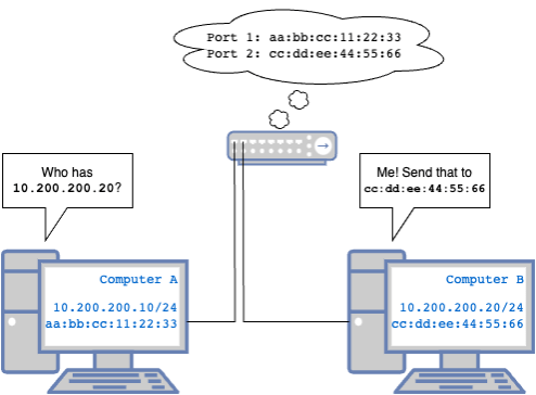
Computer A: *Hey, I need to send something to 10.200.200.20, that looks like it’s on the same network as me, but I don’t know who that is.* Hey everyone who can hear! Who is 10.200.200.20?
Computer B: *Oh hey, they’re looking for me!* Hey, that’s me, cc:dd:ee:44:55:66, you can send that over here.
Computer A: Cool. Here’s some data. I’ll remember how to find you, but if too much time passes and we haven’t spoken, I’m going to ask again.
Switch that the computers are plugged into: *Silently keeps track of what MAC addresses are sending traffic from what ports, so when computer A sends that data, it knows what port to send it to for Computer B to get it. This is sometimes called a CAM (Content Addressable Memory) table. *
So how did all that happen? Let’s start with the difference between an IP address and a MAC address. An IP address is what’s called a logical address. That is, it is defined in software and used by software. Applications on a computer listen for traffic on and send traffic to IP addresses. A MAC address, conversely, is a physical address, meaning it represents the actual physical network interface card (NIC) of the computer. Computers listen for traffic on and send traffic to MAC addresses. The NIC is the bridge that ties an IP address to a MAC address.
That initial “who has this IP address?” is called an ARP Request. ARP stands for Address Resolution Protocol and is a special type of message computers send to figure out which physical destination should receive traffic for a given IP address. When Computer B receives an ARP request for an address it holds, it replies saying “That IP is at this MAC.”Both the computer that sent the ARP request and the computer that replies will keep track of the MAC and IP address on the other side in a local database called an ARP Table. This table can be used when sending future traffic to prevent needing to have to send additional ARP requests. An entry in the ARP table is considered valid for a given length of time. This timer restarts every time traffic is received from that entry.

Computers generally aren’t plugged directly in to each other, however. They generally connect into a piece of network equipment called a switch. A switch is a device made up of multiple switchports. When a computer’s NIC is connected to a switchport, the switch starts observing which MAC addresses are originating traffic on that port. They track this information in a database called a CAM (Content Addressable Memory) Table which is often referred to as a MAC table. Computers send data through switches in units called frames. A frame is a special construct that wraps the actual important data, called the payload with some additional information the switch uses to process the frame. Think of a frame as like this message note. The actual message (the payload) goes in the large message area, and the sections above (the header) tell who the message is from, who it’s for, what type of message it is, etc. When a switch receives a frame from a computer, it looks at the destination field on the frame, which contains a MAC address. It looks at the CAM table to see if it knows about that MAC address. If it has a record of that MAC address being connected to a specific port, it will forward the frame out of that particular port. If it doesn’t yet have a record of that MAC address, it will forward the frame out to all active ports except the one it originated on, in a process called flooding. When a computer receives a frame destined for its own MAC address, it unpacks it and looks at the message inside.
There is a special MAC address called the broadcast MAC that means “send this frame to everyone on the same network.” That ARP request earlier was sent to the broadcast MAC, ff:ff:ff:ff:ff:ff. When a switch receives a frame destined for the broadcast MAC, it forwards it out all switchports in the same network. This method of broadcasting is how Computer A is able to ensure that its request made it to Computer B, but that broadcast only works if the device that needs to receive it is in the same network. With the ARP process completed, Computer A can send data with a label on it that says it’s destined for physical address cc:dd:ee:44:55:66 with the information meant for 10.200.200.20, and the switch forwards the data so it will get where it needs to go. We’ll cover how the computer decided that the IP address was on the same network in the next section.
By default, all switchports on a switch are on the same network, so every computer connected to a switch can send traffic to every other computer on a switch. IEE802.1Q (often called Dot1q), defines a standard for separating single physical network into multiple virtual networks using a construct called a VLAN (virtual local area network.) VLANs are numbered between 1-4094. A frame is placed on a VLAN in a process called tagging. A frame is tagged to a VLAN by adding an 802.1Q header specifying the VLAN to the frame between the source MAC and the Ethertype. How untagged frames are treated depends on the type of switchport the frame is traversing, that is, whether the port is an access port or a trunk port.
An access port is a switchport that is assigned to a specific VLAN. You will often see configuration such as:
interface Ethernet0/1
 switchport mode access vlan 123
This configuration defines that this switchport is solely assigned to VLAN 123. On most vendors, all ports are considered access ports unless otherwise specified, and all access ports are assumed to be VLAN 1 unless otherwise specified. Any frames received on that port are assumed to be on that VLAN. Any tagged frames are un-tagged and assumed to be on the configured VLAN, regardless of the VLAN in the tag.
A trunk port is a switchport that is a switchport that can accept traffic on multiple VLANs. Trunk ports will also have a native VLAN, which defines what VLAN untagged frames are assumed to be on. Trunk port configuration often looks similar to:
interface Ethernet0/2
 switchport mode trunk
 switchport trunk encapsulation dot1q
 switchport trunk allowed vlan 1, 2, 3, 10-20
 switchport trunk native vlan 10
This configuration defines the switchport as a trunk port using the dot1q standard1 which will allow frames tagged with VLANs 1, 2, 3, and 10-20 inclusive. Any untagged frames will be placed on the native VLAN, 10. Most switches require you to also specifically create the VLAN with a simple vlan 10 statement, for example, to create VLAN10. VLANs can be given names, but those names are generally only locally-specific descriptors to make the purpose of the VLAN more apparent when looking at the configuration or the output of diagnostic commands.
When a switch receives a frame on a given VLAN, it will only consider switchports assigned to the same VLAN, and their MAC addresses, when processing the frame. Because of this separation, computers in two different VLANs cannot talk to each other without something to bridge the gap, a process we called routing which we will talk about later. And as we already discussed, computers within the same VLAN can find each other via ARP in order to communicate with each other.
48 ports should be enough for anyone.
Multiple switches can be connected together, as well, to form larger networks. The most common way is simply by connecting switchports on two switches, generally via a trunk port. When connecting switches together, it is vitally important that one avoids creating “loops”. If a loop is created, broadcast traffic can repeat infinitely throughout the loop, eventually overwhelming the switches and causing outages. Connecting switches together in a redundant manner, however, almost invariably results in potential loops. Because of this, a family of protocols called spanning tree protocols exist. Spanning tree protocols run on all of the switches connected together and exchange information about VLANs and paths. Spanning tree then elects specific ports to act as forwarding ports which are allowed to pass traffic for a given VLAN and blocking ports which are prohibited from passing traffic for a given VLAN. These blocking ports effectively eliminate potential loop paths. There are multiple spanning tree protocols, and each works a little bit differently.
You can also “bundle” multiple switchports together to increase the bandwidth between two switches without risking loop creation. This is called link aggregation. There are multiple standards that exist for link aggregation, but the widely accepted cross-vendor standard is Link Aggregation Control Protocol (LACP.) With LACP, you can bundle switchports in groups of 2, 4, or 82. A LACP bundle acts as a single logical connection with the aggregate bandwidth of all the links in the bundle. Traffic is load-balanced across the links by way of a hashing algorithm. There are multiple ways this can work but the basic version is that all traffic between two given MAC addresses will always traverse the same link. This means that, even though a LACP bundle may have, say, 4 Gigabit ports, any given ‘conversation’ only has access to the bandwidth of the single port it was hashed to. By default, LACP bundles are confined to a single switch. However, methods exist that allow LACP bundles to span across multiple switches. This is referred to as Multi-Chassis Link Aggregation Protocol (MLAG or MC-LAG). There is no standard implementation of MLAG, so most vendors have their own proprietary implementation. Cisco’s Nexus platform implements this via Virtual Port Channel (VPC), and Arista’s implementation is simply referred to as MLAG.
There is also another concept where two physical switches can be combined into one larger logical switch, allowing them to be configured as a single unit. This is often called virtual chassis or switch stacking. This works by connecting the switches together with special high-bandwidth connections. These can either be proprietary dedicated ports or by re-purposing existing high-bandwidth switchports. The individual switches are configured to participate in the logical switch cluster, and generally one individual physical chassis will act as the “primary” that manages the cluster.
Networks have layers. Like an ogre.
We’ve talked about frames pretty extensively so far, but more than likely, when talking about computers communicating, you probably hear the word packet. We traditionally talk about packets because software sends and receives packets and routers route packets. When a piece of software on one computer needs to send that packet to another computer, that packet ends up in a frame. This process is best understood by way of the concept of network layers. There are different ways people organize the network into layers, but you will most often hear about the OSI Model, so let’s use that one.
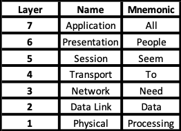
The OSI Model is a way of breaking down computer applications into 7 components: Application, Presentation, Session, Transport, Network, Datalink, Physical. A common mnemonic for remembering these is “All People Seem To Need Data Processing”. We’re going to take a moment to describe the layers we need to know about and help form a connection to a concept we already understand: talking!
NOTE: As I’ve been editing this, I’m skeptical of my analogy’s cromulence. I will almost certainly be revisiting this.
Physical Layer
The Physical layer (or layer 1) is exactly what it sounds like: the physical aspects of a network responsible for the transmission of electrical (or optical) signals. Ultimately, all data between sent between computers is reduced to binary, and those binary 1s and 0s are transmitted as electrical signals. The NIC, physical cabling, and switch port participate in the physical layer and are responsible for carrying these electrical signals.
The analog for us would be the lungs, vocal cords, mouth, the air itself, and our ears. Lungs pass air over the vocal cords, which vibrate the air producing sound waves. Our mouths further shape the air and resultant sound waves, and our ears pick up the soundwaves via our ear drums.
Data Link Layer
The Data Link layer (or layer 2) is responsible for modulating data into an electronic signal that can be carried by the physical layer, as well as demodulating electronic back to data3. This modulation and demodulation provides the means for entities to communicate across physical medium. The two most common layer 2 protocols are IEEE 802.34 (you’ve heard of this as Ethernet) which defines wired networking, and IEEE 802.11 (a family of protocols with the catchy marketing term Wi-Fi) which defines wireless networking. The terms MAC address, physical address, and layer-2 address are synonymous. Switches are layer 2 devices, and VLANs are layer 2 boundaries. Data at the Data Link layer is organized into frames. NICs and switch ASICs bridge the physical layer to the data link layer.
The analog for us would be the portions of our brains that control our vocal cords to vibrate sound in specific ways, as well as the portions that receive nerve impulses from our ears and process the sound. An analog to a layer two protocol would be the letters and their sounds, as well as how to combine sounds to form words with specific meanings. That is, I can take the word “dog” and generate the correct nerve impulses to move the air correctly to generate the right sound, and your ear, having sent the sound to your brain, can process that sound and convert it back into the word “dog”. We have shared data, but not truly communicated yet.
Network Layer
The Network layer (or layer 3) provides additional options and capabilities to this communication. While the data link layer and physical layer facilitate the conversion and transmission of data between directly connected hardware via electronic signals, network layer protocols facilitate communication between software, including the capability of routing communication between devices on different networks. The most common layer-3 protocol, and the one we will focus on in this material, is IP (Internet Protocol), but ICMP (Internet Control Message Protocol) and IPsec (Internet Protocol Security) and ARP (Address Resolution Protocol)5 are also Layer 3 protocols, and data at the network layer is organized in units called packets.
The human analog here is grammar and syntax! These are the rules for forming sentences and paragraphs, with punctuation and parts of speech. Now we aren’t just shouting words at each other, we are able to convey ideas.
Transport Layer
The Transport layer (or layer 4) formalizes the rules that applications will follow when communicating via the network layer. A layer 3 protocol by itself merely defines the “language” but does not provide for rules of how conversations are meant to occur. Transport layer protocols, such as Transmission Control Protocol (TCP) and Universal Datagram Protocol (UDP) define the rules for a conversation.
TCP is what is called “connection-oriented” and is for a two-way dialogue. Both ends communicate back and forth, acknowledging the receipt of one piece of information and readiness to receive the next, the same way that two people would sit and have a conversation. TCP is used when verifying the integrity of the data passed back and forth is important enough to slow down the conversation to allow for error handling and correction.
UDP is what is called “connectionless”, the same way a radio broadcast is just sent out, with no concern for whether or not it is actually heard. UDP is used when it is more important for the data to receive the destination as fast as possible and lost or out-of-order packets are not necessarily fatal. UDP is often used for streaming video and audio.
At layer 4, we have an additional concept called ports, which are channels that an individual application can use to send and receive traffic without it getting mixed up with traffic for other applications on the same computer. Similar to how a single street address can have suite numbers to allow an individual to send/receive mail, port numbers allow multiple applications to send/receive data from a single IP address. There are well known ports that are assigned to specific protocols (such as port 80 for HTTP, port 25 for SMTP) as well as ephemeral ports that can be used in a dynamic/ad hoc fashion when only needed for a short time.
Session, Presentation, and Application Layers
The higher layers, 5-7, are very application specific. Things like HTTP, DNS, SMB, etc. These are applications and protocols whose information is contained within TCP/IP or UDP/IP packets to get the information to the right destination. It is important in general to understand more about these, but it is outside of the scope of this class.
The OSI layer is most practically useful as a troubleshooting device. In networking, it is always best6 to start troubleshooting at the physical layer and working up.
On Frames and Packets
As mentioned, a frame is the layer-2 format used to place data on the wire in Ethernet networks. However, we almost exclusively talk about packets on a day-to-day basis. If you are actually concerned with Ethernet framing, chances are you are troubleshooting a particularly annoying problem or actually designing or building a switch. However, understanding the interaction between the two is going to be helpful as we progress.
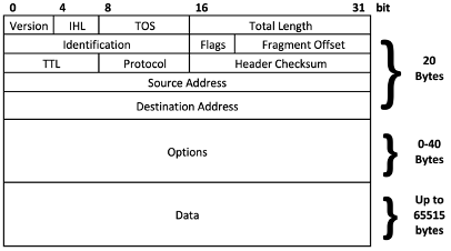
A packet is a layer-3 software construct and is how software on a computer packages data when it wants to send it to another piece of software on another computer7. Let’s take a look at IP packets. An IP Packet includes a header, options, and the payload. And remember that an IP address is a logical address, not a physical address. In fact, a single computer can have multiple IP addresses associated with the same MAC address.
The header contains vital information for handling the packet. The main ones are the source address and destination address, indicating where the packet came from originally and where it is ultimately headed. Also important, however, is the TTL (Time To Live.) The TTL will become very important when we start talking about routing and indicates the maximum distance a packet is allowed to be routed before it should be dropped. The header checksum is the result of a mathematical operation performed on the data in the packet header and is useful in ensuring the header contains the same data that was originally sent, and that no errors were introduced along the way. The other fields in the header can be ignored for the purposes of this class but become very important when discussing further advanced network topics such as Quality of Service (QoS) or when dealing with issues such as fragmentation8.
The Options field is not commonly used and can be ignored for the purposes of this material.
The Data field includes the actual payload of the packet as transmitted from the source application to the destination application.
However, when that packet needs to be sent somewhere, it needs to be placed inside a frame before it can be sent on the wire. This preparation happens through a process called encapsulation. Encapsulation takes an IP packet and makes it the payload to an ethernet frame. The Ethernet frame is then headered with the source and destination MAC address, providing the information required to physically transport the packet to the switch where it can be forwarded based on the destination MAC address based on the switch’s CAM table. An Ethernet frame looks like this, with our IP packet being the payload of the frame.

Software cares about packets, hardware cares about frames. When a computer sends a packet, the NIC encapsulates it in a frame. When a NIC receives a frame, it decapsulates the packet for the software. This will be important later. So really what happened in the above example was “The software on computer A generated an IP packet, the NIC on computer A encapsulated that in an ethernet frame.” I will use packet most of the time, specifying frames when they are important. If you want to learn more about this in detail, look up ethernet, frames, and encapsulation.
Let’s talk about network devices briefly. There are, broadly speaking, three basic network devices that correlate to layers 1, 2, and 3:
- Hub – A layer 1 device. Also sometimes called a “Repeater Hub”, a hub is a very simple device that takes in traffic on one port and, instead of intelligently finding out which port it is destined for, instead sends the traffic out on all ports. Naturally, this generates a lot of extra traffic by not intelligently limiting where to packets.
- Switch – Traditionally a layer-2 device. A switch adds intelligence by keeping track of what MAC addresses can be found beyond specific ports, and only sends traffic where it needs to go. Switches can be logically segmented into multiple network segments called Virtual Local Area Networks, or VLANs to isolate traffic as needed.
- Router – A router is used to allow traffic from one layer-2 segment to be routed to another layer-2 segment. Routers have multiple interfaces that act as legs into different layer-2 segments to facilitate passing traffic from segment to segment. Routing operates at layer 3 and relies on the IP address to make the decision on where to send traffic. The information used to make these decisions is called the routing table. Some switches are what is called a Layer-3 Switch and integrates routing. We’ll talk about routing next!
Four main types of traffic
There are four main classifications of traffic based on the intended destination. These are Broadcast, Unicast, Multicast, and Anycast. These classifications exist at both layer 2 and layer 3.
Unicast Traffic
Unicast traffic is traffic that has a single specific destination. A unicast packet will have a specific host IP address in the destination and will be encapsulated in a unicast frame with the associated destination MAC address. There is also a concept called Unknown Unicast, where a frame is destined to a MAC address that the switch does not already have in the CAM table. This results in the switch flooding the frame to all ports.
Broadcast Traffic
Broadcast traffic is traffic destined to every host in the broadcast domain. A broadcast domain is generally defined by layer 2 boundaries (A single VLAN or multiple VLANs joined by network encapsulation such as VXLAN). The broadcast MAC, we learned earlier, is ff:ff:ff:ff:ff:ff. Frames sent to the broadcast MAC are flooded to every port in the VLAN.
Multicast Traffic
Multicast traffic is a rather complex topic that we do not need to get into the details of, so a brief summary will suffice. In short, multicast is traffic destined to a every member of a specific group of endpoints. There are special multicast IP addresses in the range of 224.0.0.0 to 239.255.255.255, and special multicast MAC addresses in the range of 01.80.C2.00.00.00 to 01.80.C2.FF.FF.FF. Hosts can “subscribe” to a specific endpoint tied to a specific IP. Any traffic destined for that IP will be forwarded to all subscribed hosts. A common use for this is in phone systems with music-on-hold. A single “music-on-hold” device will broadcast a single stream of the music to a multicast IP, and phones can subscribe to that multicast IP to receive the music-on-hold stream. This greatly reduces the amount of traffic that would be required for an individual stream to be sent from the music-on-hold device directly to each phone. We do not need to delve any further into Multicast for this class, but knowing it exists and why it exists will be helpful.
Anycast Traffic
Anycast traffic is also a rather complex topic that we can avoid the details of, but the Anycast concept is used in NSX and Flow. Anycast is a methodology where a single IP address is shared by multiple endpoints, and any one of those endpoints, generally the closest one, will pick it up. This will make a little more sense once we cover Network Encapsulation later, but a typical use of this is in a spine-and-leaf architecture where VXLAN is used. Each switch with a given VXLAN configured can also listen for traffic for the default gateway for the VXLAN. This reduces the traffic that needs to traverse the spines in order to reach the default gateway, as it can always be made local. In NSX and Flow, each hypervisor acts as an Anycast gateway for the same purpose.
BUM Traffic
“But you said there are only 4 types of traffic!” Yes. BUM traffic means “Broadcast, Unknown Unicast, and Multicast Traffic.” In these three scenarios, the switch generally doesn’t know where the destination MAC can be found, and therefore ends up having to flood the frame. Because of this, these are often discussed as the aggregate, BUM traffic.
A quick note about MAC addresses
MAC addresses have two portions. These are the Organizationally Unique Identifier (OUI) and the NIC-Specific Identifier. The OUI identifies the manufacturer (or software in the case of virtual NICs) responsible for creating the NIC, and the NIC-Specific Identifier is unique to the particular NIC for that OUI. There are also ways to identify whether a MAC is physically assigned or logically assigned, or whether they are multicast or unicast. This information can help you quickly identify, for instance, VMWare vNIC MACs when looking at an ARP table or MAC table but will not be covered in this class. For more details, the Wikipedia article on MAC addresses is an excellent resource.
- Cisco had a proprietary VLAN standard called ISL (Inter-Switch Link.) ISL is no longer in use anywhere that matters. Because of this, many versions of Cisco IOS require you to define the vlan encapsulation mode. ↩︎
- Yes, you can create a LACP bundle with a non-power-of-2 quantity of interfaces, but that is not best practice, as the algorithm that determines which link a frame takes will not work efficiently or correctly. ↩︎
- Fun fact: this is where the term “Modem” originates, as a blend word of Modulate/Demodulate, as that is what they did! ↩︎
- IEEE (pronounced I-Triple-E) is the Institute of Electrical and Electronics Engineers, a non-profit group that defines and coordinates standards for electronics around the world and is made up of families that focus on various topics. IEEE 802 is focused on LAN (local area network), PAN (personal area network) and MAN (metropolitan area network) technologies. Sometimes, standards defined by the IEEE are referred to by their IEEE number, and sometimes they have more common names. Since layer 1 and layer 2 protocols define how data is physically transmitted, it is the IEEE that has defined these standards. Higher layer protocols and standards are defined by the IETF (Internet Engineering Task Force) in documents called RFCs (Request For Comment), so you will sometimes see references to standards by their RFC number, such as RFC 1918 that defines private IP addressing. ↩︎
- When I was a young child, ARP was considered a layer 2 protocol. Modern texts will often place it in layer 3, or if they feel like being especially confusing, describe it as “layer 2.5”. Conceptually, I believe it makes the most sense to think of it as a layer 3 protocol, but my feelings on the topic are not strong enough that I’d argue with you if it makes more sense to you as a layer 2 protocol. ↩︎
- One might hear the word “best” and think: “Well, that sure sounds subjective! Surely this is merely opinion.” And in most cases, I would agree that my determination of what is best is merely my opinion. Dear reader, in this case, I am declaring my opinion to be objectively correct. Martin’s Razor states that “Any instance where troubleshooting is started at a higher layer guarantees that the issue will be found at a lower layer.” Even in virtual networking, always check the physical first. ↩︎
- Packets can also be used when one piece of software is sending data to another piece of software on the same computer. For instance, if a computer has an application and a database, the application will often communicate to the database via IP using a special IP address, 127.0.0.1, called a loopback, and often referred to as localhost. Packets sent to 127.0.0.1 are processed by the local computer, passed between one port and another. ↩︎
- Notice that an IP packet can be upwards of 65000 bytes. Frames are generally limited to approximately 1500 bytes. Fragmentation can allow a single packet to be broken up into multiple frames. ↩︎
